A Composite Score System (CSS) instead of the Net Run Rate (NRR) - The 2021 ICC T20 World Cup

At the time of writing, the 2021 ICC T20 World Cup is finally over. Four teams qualified for the semi-finals – two each from the two groups of six teams that played in round-robin fashion in what is called a Super 12 stage. The teams were chosen from each group for having gained the most points based on a scoring system that assigns two points for a win. There was no problem with Group 2 – Pakistan topped with 10 points from all the 5 matches they won and New Zealand had 8 points from the 4 matches they won, having conceded only to Pakistan. The problem with this simple scoring system, 2 points for a win irrespective of how close the match had been, was that in Group 1, three teams were identically tied on 8 points each – Played 5, Won 4, Lost 1, No Result 1 and 8 points. Each team lost one match in a classic Win-Loss loop: South Africa > England > Australia > South Africa, with the > sign indicating the direction of the win. To resolve this tie and choose only two teams, the Net Run Rate (NRR) was computed, and this calculation favoured England (2.464) and Australia (1.216) at the expense of South Africa (0.739). As a metrician I find this unsatisfactory for reasons I shall state below.

This tie is resolved with another controversial ICC rule – The Net Run Rate (NRR) criterion. It depends only on runs scored off balls delivered to the team and not at all on how many wickets they have lost in the course of the match. Here, I shall use the count of balls instead of overs for the finer granularity it offers.

The NRR is based on what is called a batting strike rate. The higher the batting strike rate is for an individual batsman, the more effective he is at scoring quickly. In Test cricket, it is usually understood that a batsman's strike rate is of less importance than his ability to score runs without getting out, i.e., without losing his wicket. Thus, in Test cricket, a batsman is evaluated on his batting average, rather than on his strike rate. At the same time, a player's bowling average is the number of runs they have conceded per wicket taken. The lower the bowling average is, the better the bowler is performing. It is not the economy rate, which is the average number of runs conceded per over bowled. NRR ignores the former aspect and gives importance only to the latter.

Extending this argument to ODI and T20 team events, one should think that NRR is only a partial evaluation of a team’s performance. Equally, if not more important perhaps is one team’s ability to score without losing wickets, and the opposing team’s ability to seize wickets before the run chase gets over. Let us illustrate this idea with some toy examples. First, let us see what happens when Team X batting first in a T20 match scores 200 runs (RX) off exactly 20 overs (i.e., 120 balls, or BX) without losing a wicket (w = 0). Team Y chases this total and manages a win by scoring 201 runs off the same number of balls, but only after surrendering 9 wickets (w = 9). All 2 points for a win are awarded to Team Y. The RR calculation for this is (R/B)X – (R/B)Y = 200/120 – 201/120 = -0.083 for Team X, and by an inversion of the same logic, a RR score of 0.083 for Team Y. Note that a difference is taken. This is crucial to the argument that follows, where for the CSS we do not take a difference but consider what is called eigenvector centrality from a matrix with entries in rows and columns. The NRR is the sum total of all these differences, for all the matches played by a team. The only other complication is that if a team is all out before its stipulated overs are bowled, then a default of 120 balls is applied to their RR calculation.

In our proposed composite indicator, we take into account a score for the number of wickets lost by the batting team (i.e., taken by the bowling team). Here some subtlety is required. If no wickets are lost, as in the case where Pakistan overtook India’s total without losing a wicket, we start the count with one. This helps us to avoid a division by zero. And if w wickets are taken, the count for this is W = w + 1. This is fair; when all wickets are down, i.e., w = 10, there have been 11 players at the crease, for W = 11. Thus R/W becomes a second indicator for performance and is the team’s equivalent for batting average. Thus, we have to contend with two indicators, R/W and R/B, with different units, namely runs/wicket and runs/balls. It is known in physics (a wise man once said that physics is all about counting rules), that disparate units cannot be added (that is oranges and apples cannot be added). But they may be combined by multiplication. The composite score system (CSS) thus gives CS = (R/W) x (R/B). Let us apply this counting rule to the example above. Team X gets CSX = (200/1) x (200/120) = 333.33 and for Team Y, we have CSY = (201/10) x (201/120) = 33.67. These will be entries of cells in a matrix corresponding to the rows and columns for Teams X and Y. We do not take differences! Note the huge disparity in scores: 333.33 vs 33.67. This reflects the reward for the bowlers from Team X who managed to remove 9 batsmen from Team Y, where their counterparts from Team Y could not succeed even with one. That is, X outplayed Y in both batting and bowling and yet lost the match.

The second example we take will be to see what happens if Team X batting first pulls off a dramatic win. Let us say Team X scores 200 runs (RX) off exactly 20 overs (i.e., 120 balls, or BX) but loses all 10 wickets (w = 10, or W = 11). Team Y chases this total but loses, scoring 199 runs off the same number of balls, but without losing a single wicket (w = 0, or W = 1). All 2 points for a win are awarded to Team X. The RR calculation for this is (R/B)X – (R/B)Y = 200/120 – 199/120 = 0.083 for Team X, and by an inversion of the same logic, a RR score of -0.083 for Team Y. This is because differences are taken. The composite score system (CSS) gives Team X, CSX = (200/11) x (200/120) = 30.30 and for Team Y, we have CSY = (199/1) x (199/120) = 330.01, and these go as entries for the cells AXY and AYX respectively, corresponding to the rows and columns for Teams X and Y. Now, the huge difference in scores 30.30 vs 330.01, rewards the bowlers from Team Y who managed to remove 10 batsmen from Team X, where their counterparts from Team X could not succeed even with one. That is, Y outplayed X in both batting and bowling and yet lost the run chase and hence the match. But this is the spectacle that fans want.

So far, we have argued that NRR based on differences of strike rate gives an incomplete understanding and that the Composite Score which also accounts for the batting rate together with the strike rate gives a better handle on performance evaluation. Note that when two teams meet, each team earns points, and these should actually populate the cells of a two- dimensional matrix. To a metrician, the differences we are considering are based on the row- sums and column-sums of the matrix. A better picture is obtained if we actually investigate a property of this matrix known as eigenvector centrality. It is best to illustrate this with some real-world examples from the 2021 ICC T20 World Cup.

On 11-Nov 2021, in the second semi-final, the winner of Group 2, Pakistan played Australia, the second placed team in Group 1. Pakistan scored 176 runs in 20 overs, losing 4 wickets.

Australia won the run chase and the spot in the final by scoring 177 runs for the loss of 5 wickets but with an over to spare (i.e., in 114 balls or 19 overs). The CS score for Pakistan was (176/5) x (176/120) = 51.63 and that for Australia was (177/6) x (177/114) = 45.80. The CSS scheme gives the match to Pakistan! Note that by ICC rules, in the other semi-final, the winner of Group 1, England lost to the second placed team in Group 2, New Zealand. Thus, at the knockout stage, we have another Win-Loss Loop: Pakistan > New Zealand > England > Australia > Pakistan. We shall see next how Ramanujacharyulu’s power-weakness tournament metaphor using graph theoretical techniques will get us out of such traps.

I have written elsewhere (see some old issues of Science Reporter) about an Indian mathematician named Ramanujacharyulu (C. Ramanujacharyulu, Analysis of preferential experiments, Psychometrika, 3 (1964), pp. 257-261) who more than a half-century ago, introduced a paired-comparison protocol based on graph theory which allows us to reconcile the results of all the teams and their matches in a round-robin tournament. Ramanujacharyulu (henceforth Ram) tried to find out who can combine the greatest ability to win with the least susceptibility to lose. That is, "in tournaments one may be interested in locating the really talented man (sic) in the sense that he has won over the largest number of opponents but simultaneously he has been defeated by only a few opponents."

Let us look at Group 1, where three teams were identically tied on 8 points each. Each team lost one match in a Win-Loss loop: South Africa > England > Australia > South Africa, with the > sign indicating the direction of the win. Instead of resolving this tie to choose two teams, on the Net Run Rate (NRR), we shall examine how we can proceed with Ram’s graph theoretical logic.

For each of the 15 matches played in round-robin style Group 1, we can compute CS scores as a pair, and these can be arranged in matrix form as shown in Table 1. The calculations can be easily performed using Excel operations and the Excel spreadsheets are available from this author on request. The table at top is called the Power matrix, and the rows give the CS scores “for” each team and the columns give the CS scores against “each” team. The inverse of this matrix is also shown in Table 1 as the Weakness matrix. As an illustration, on 04-Nov 2021, where Bangladesh v Australia produced the scores 73 (15 overs) v 78/2 (6.2 overs), we get (73/11) x (73/90) = 5.38 and (78/3) x (78/38) = 53.37. These are the entries seen at the second cell in the first row (Australia v Bangladesh) and the first cell in the second row (Bangladesh v Australia).

The row-totals or row-sums (let us call this P) give an idea of the “power” of each team and the column-totals or column-sums (we will call this W) give the “weakness” of each team. From a graph theoretical perspective, ICC uses RR scores instead of CS scores at these locations and takes the difference of the row-sums and the column-sums as a measure of performance of each team. If we apply Ram’s protocol to the CS scores, then we have a more complete assessment of the relative merits of the teams when they play each other – in simpler words, while the attacking record is rewarded, the defensive role is also credited. The P values (i.e., the row-totals) and the W values (the column-totals) now measure the “power” and “weakness” of each team. The P/W ratio (we call this the Power-Weakness Ratio) and the ratio (P-W)/(P+W) (we shall call this the Normalized Power-Weakness Difference) are dimensionless measures of the “quality” of the team. Note that PWD is a one-to-one monotonic transformation of PWR. PWD has the attractive feature that it is always bounded between -1 and 1 but this is not true of PWR which has no upper bound. In Table 1, we see that Australia has the best power score (the higher, the better) and South Africa the best weakness score (that is the lower, the better).

At this stage, we should understand that the simple row-sums and column-sums assume that each team is given the same weight. Thus, South Africa gets the same weight for a win against England as it would for a win against West Indies. Ramanujacharyulu pointed out that the weightage can be changed iteratively, taking into consideration the “quality” of the team, leading to an eigen-value problem. (In graph theory, we are using eigenvector centrality (also called eigencentrality or prestige score) as a measure of the influence of a node in a network. Relative scores, or weights, are assigned to all nodes in the network based on the idea that connections to high-scoring nodes contribute more to the score of the node in question than connections to low-scoring nodes. A high eigenvector score means that a node is connected to many nodes who themselves have high scores.) Effectively, this is done by multiplying the citation matrix by itself recursively until convergence is reached in both the power and weakness dimensions. This yields the weighted values of P (k) and W (k) and the ratio of these values is PWR (k), where k is the number of iterations required to achieve convergence. This graph-theoretical procedure has considerable mathematical elegance: it handles the rows (power) and columns (weakness) symmetrically although the matrix, to start with, was necessarily asymmetrical.

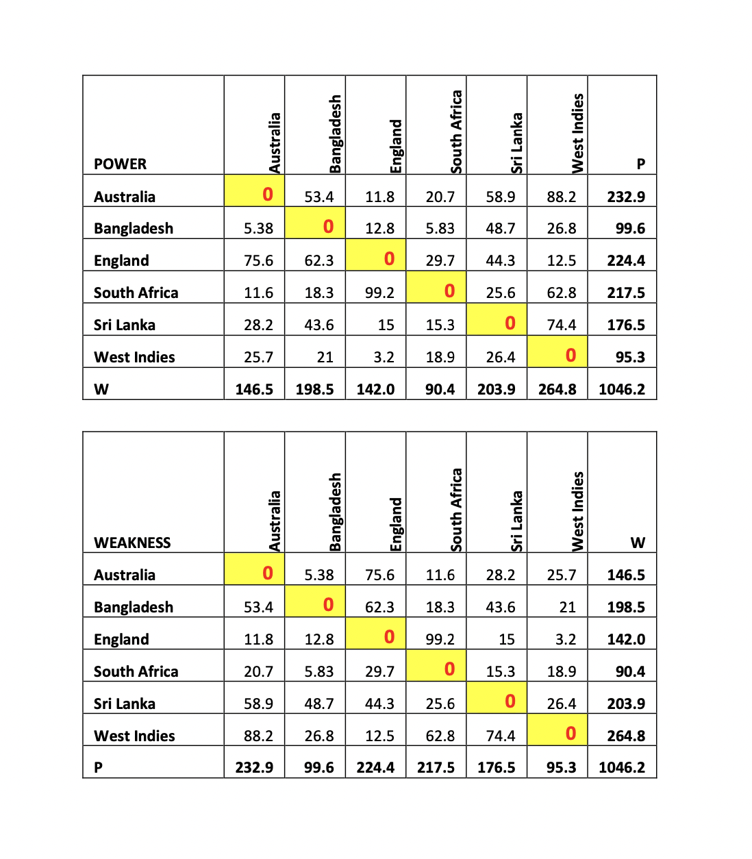
Table 1 shows the matrix position of all the teams at the end of the round-robin stage on 6th November 2021 for Group 1.

Fig. 1 shows the two-dimensional dispersion of Power-Weakness Ratio (PWR) and Normalized Power-Weakness Difference (PWD) for the tournament matrix for the Group 1 round-robin stage before iteration starts. Note that this clearly brings out the one-to-one monotonic correspondence between the PWR and PWD scores. Australia and England are for all practical purposes very closely tied at the second and places. We found that after recursive iterations corresponding to the weighting logic, there was acceptable convergence after 12 iterations. In Fig. 2 we report the final standings and how PWD (12) relates to PWD (1) for Group 1. Weighting has made a difference to the relative rankings of England and Australia with the former having clearly pulled away. Ram’s tournament metaphor protocol has found a way out of the dilemma of the Win-Loss loop. Thus, it is South Africa and England that should have gone to the knockout stage. ICC’s NRR is more like a lottery, and it is time ICC replaced it with a more rational system like the Ramanujacharyulu protocol. The CSS approach gives finer granularity than the row-wise count of wins and this combined with Ram’s graph theoretical computations gives an unambiguous result.

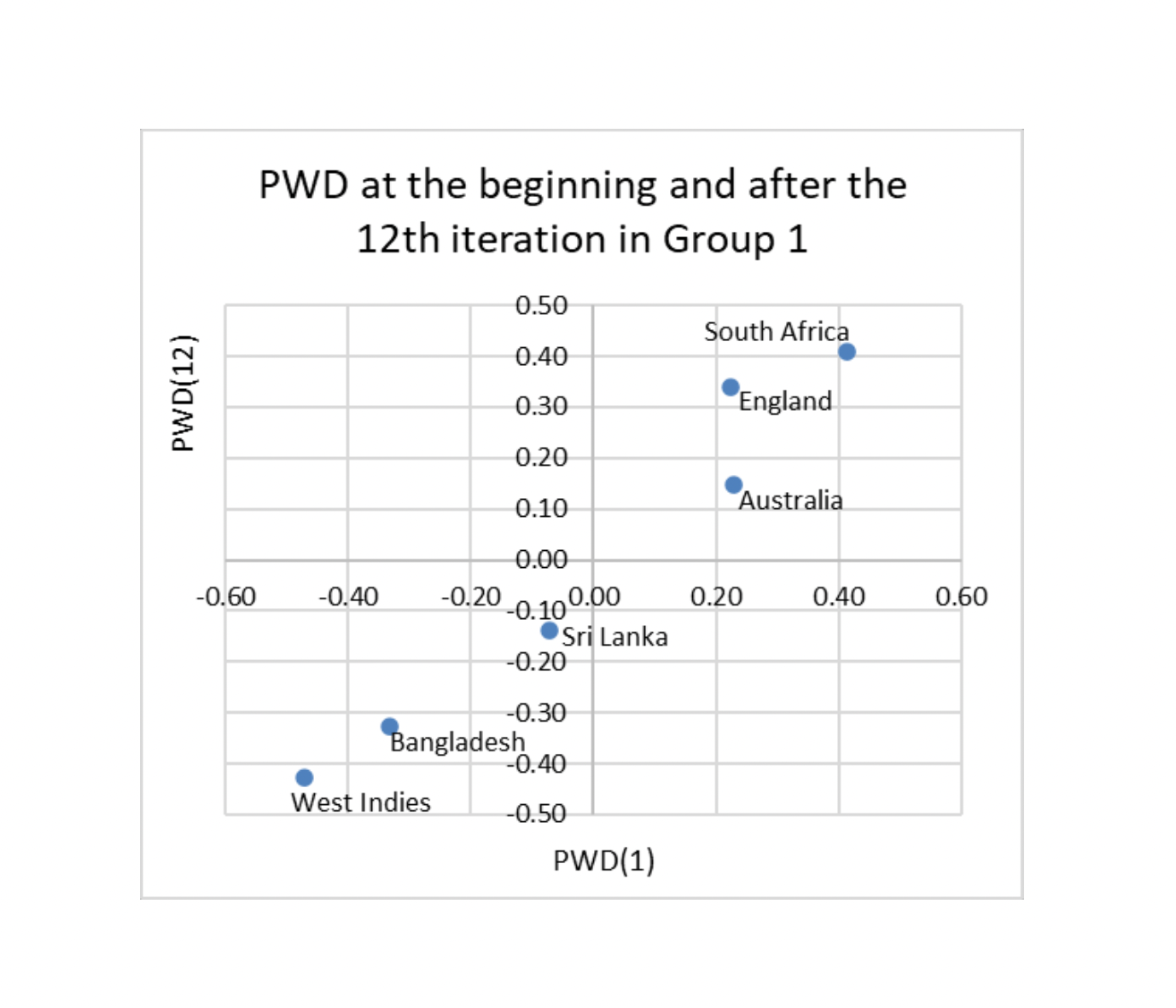
Fig. 2 shows the relative two-dimensional dispersion of Power-Weakness Difference (PWD) scores before iteration, and after 12 iterations for the Group 1 round-robin stage. Weighted iteration has allowed England to pull away from Australia.

We shall not elaborate on Group 2 as there were no Win-Loss conflicts. Instead, we will go to the final standings after three more matches were played in the knockout stage: two semi- finals and a grand final. Again, we use the CSS paradigm and assemble a matrix of all 12 teams. Table 2 shows the power matrix position based on CSS values of all the teams at the end of the tournament on 14th November 2021. The knockout stage matches are highlighted as shown. The weakness matrix is just the inverse of this matrix.

The recursive iterations are continued as before and in Fig. 3 we report the final position. Note that all teams have not played the same number of matches. While 8 teams have played 5 matches each, two teams have played 6 matches each and the two teams in the final have played 7 matches each. This is not an issue because the performance parameter PWD is a dimensionless ratio. The relative two-dimensional dispersion of Power-Weakness Difference (PWD) scores before iteration, and after 12 iterations for all teams finally on 14-Nov 2021. produce some interesting results. Weighted (i.e., recursive) iteration takes South Africa to the top position while if recursive iteration were not used, then it is Pakistan that took this place.

Fig. 3 shows the relative two-dimensional dispersion of Power-Weakness Difference (PWD) scores before iteration, and after 12 iterations for all teams finally on 14-Nov 2021. Weighted (i.e., recursive) iteration has allowed South Africa to reach the top position while if recursive iteration were not used, then it is Pakistan that took this place.

Table 2 shows the power matrix position of all the teams at the end of the tournament on 14th November 2021. The knockout stage matches are highlighted as shown.

To sign off, a prayer. Let the fans award go to Australia, as this is the spectacle that viewers in the grounds and across the world want, but surely the sports analysts’ award based on computational data analysis must go to South Africa.

The author is thankful to P Jafarali, a cricketer and fan himself, for a very careful reading of the early drafts and for many insightful comments.